Load Frequency Control (LFC) & Turbine Governor Control (TGC) in Power System

Brief Introduction to Thermal Generating Units

Electricity generation relies on both renewable and non - renewable energy resources. Thermal generating units represent a conventional approach to power production. In these units, fuels such as coal, nuclear energy, natural gas, biofuel, and biogas are combusted within a boiler.

The boiler of a generating unit is an extremely complex system. In its simplest conception, it can be visualized as a chamber whose walls are lined with pipes, through which water continuously circulates. The thermal energy liberated by the combustion of fuel inside the boiler is transferred to this water. During this process, the water is transformed into dry saturated steam characterized by high pressure (ranging from 150 ksc to 380 ksc, depending on the design) and high temperature (between 530°C and 732°C, subject to design specifications).

This saturated steam is then fed into a turbine, where it expands and its temperature drops. In this expansion process, the steam transfers its thermal energy to the rotational energy of the turbine shaft. The flow of steam into the turbine is regulated by a control valve, which is governed by the turbine's governing system. Consequently, the active power output of the turbine is controlled by the governor. The turbine is coupled with a synchronous generator.

The synchronous generator converts the mechanical energy of the turbine into electrical energy. Synchronous generators produce electricity at relatively low voltages, typically in the range of 11 kV to 26 kV, at the nominal frequency. This voltage is then stepped up to 220 kV/400 kV/765 kV by a generating transformer for transmission into the power grid. In power system studies, this entire integrated system is referred to as a generating unit.

Turbine Governor Control (TGC)

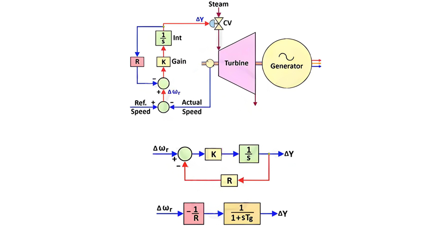
As previously mentioned, the governor regulates the active power flow into the turbine by controlling the position of the control valve. A hydraulic governor can be modeled as an integral controller that takes feedback from the turbine’s actual rotational speed. Figure 1 illustrates the governor’s operation in speed - control mode.

The turbine’s actual speed is compared against the reference speed (corresponding to the nominal grid frequency). The resulting speed error signal (∆ωᵣ) is then fed to the governor. Based on this error signal, the governor adjusts the control valve position: if a positive error signal is detected (indicating the actual frequency exceeds the nominal frequency), the governor slightly closes the valve; conversely, it opens the valve when a negative error signal is received.

“R” represents the governor’s droop setting, typically ranging from 3% to 8%. Mathematically, it is defined as:
R = (per unit change in frequency) / (per unit change in power)

Droop settings are critical for the stable parallel operation of multiple generating units, as they determine how load is shared within a control area. Units with a smaller droop value will automatically assume a larger share of the load.

Control Area

In a power system, generating units and loads are distributed across vast geographical regions. To maintain stability, the entire grid is divided into smaller control areas (primarily based on geography). This division enables:

Efficient load flow calculations
Precise control of frequency and power balance

Within a control area, multiple generating units and loads coexist. Subdividing the power system into control areas serves several key objectives:

1. Load Frequency Control

This framework enables the application of load - frequency control methods to maintain grid frequency—a concept explored in greater detail later.

2. Determination of Scheduled Interchanges

If a control area’s generation falls short of its load demand, power flows into the area from neighboring control areas via tie lines (and vice versa).

3. Effective Load Sharing

Load demand varies throughout the day (e.g., lower at night, peaking in the morning and evening). Control areas simplify the process of:

Allocating load across units based on projected demand and unit capacity
Calculating scheduled power interchanges with other control areas

Power Balance

Electrical energy is consumed in real - time (it cannot be stored on a large scale). Thus, power balance is a fundamental requirement:
Power Generated (P₉) = Load Demand (Pd) + Transmission Losses (Pₗ)

Transmission losses typically account for ~2% of generated power and are often neglected when focusing on frequency control. For simplicity, we approximate:
Power Generated (P₉) ≈ Load Demand (Pd)

Frequency Variation

Grid frequency fluctuates due to mismatches between load demand and generation. While minor deviations are stabilized by system inertia, significant gaps (e.g., unit trips, large load changes) can cause frequency to vary by ±5%. Key scenarios include:

Unplanned outages of generating units or transmission lines
Sudden connection/disconnection of large loads

In most cases (e.g., unit/line trips, large load connection), demand exceeds generation, causing frequency to drop. Conversely, if a transmission line serving a large load trips, generation may exceed demand, causing frequency to rise. Though the system responds oppositely to these scenarios, understanding frequency dips suffices to grasp both behaviors.

Why Frequency Dips Occur

Two inherent system behaviors drive frequency dips:

1. Load Dampening

Induction motors (e.g., household fans, industrial drives) dominate grid loads. Their power consumption is frequency - dependent: a 1% frequency reduction typically reduces active power consumption by ~2% in large systems. When new loads connect, frequency drops, and existing induction loads automatically consume less power—partially mitigating the demand - generation gap.

2. Kinetic Energy Release from Turbine - Generator (TG) Sets

Conventional TG sets have massive rotors (often >25 tonnes) spinning at 3000 RPM (for 50Hz grids). When demand exceeds generation, these rotors temporarily supply stored kinetic energy (for 3–5 seconds, depending on inertia). As rotors slow down, grid frequency drops.

Frequency Control

Load - frequency control (LFC) restores grid frequency to its nominal value after demand - generation mismatches. Two tiers of control exist:

1. Primary Frequency Control

At the unit level, the turbine’s governing system adjusts speed (and thus frequency). As shown earlier, each unit modulates steam input based on frequency deviations. The full primary control loop for a generating station is depicted in the figure below.

2. Secondary Frequency Control

This involves coordinated control across multiple units in different control areas, ensuring long - term frequency stability and optimal load sharing.

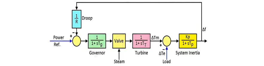
Primary Frequency Control Limitations

Primary frequency control alone results in a steady - state frequency deviation, influenced by the governor droop characteristic and load frequency sensitivity. This occurs because individual units adjust speed without considering where new loads are connected or how much load is added. Without such contextual assessment, power balance cannot be fully restored, and frequency deviation persists. Following primary control actions, the steady - state frequency error may be either positive or negative.

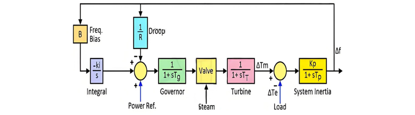
Secondary Frequency Control

Restoring system frequency to its nominal value requires secondary control, which accounts for new load locations and adjusts reference setpoints for selected units. When load increases in a control area, generation within that area must rise to:

Maintain demand - generation balance at the control area level
Keep scheduled interchanges with adjacent areas within pre - defined limits

To achieve this:

Automatic Generation Control (AGC) assigns specific units in each control area for secondary control.
A frequency bias loop is added to their control systems, providing real - time corrective signals based on load flow calculations.

Once revised load setpoints are issued, units begin adjusting generation. Due to the mechanical nature of power production, it takes 25–30 minutes for units to reach their scheduled outputs. When all generating stations achieve target generation, power balance is reinstated, and frequency returns to nominal.

The overall response of the system with the primary and secondary frequency control can be understood by the graph below.

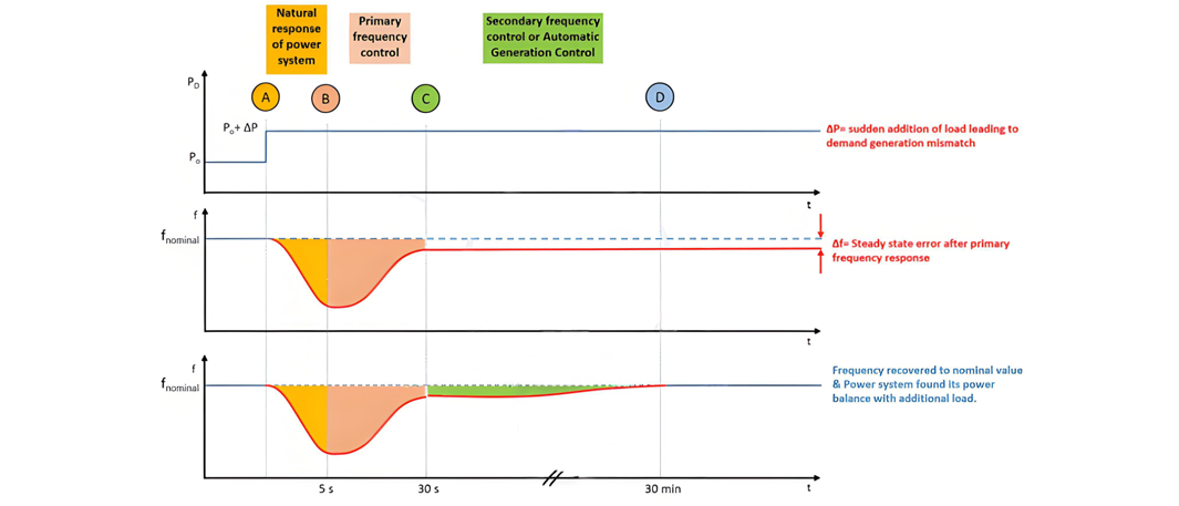
System Response to Load Increase (A-B-C-D)
A-B: Transient Kinetic Energy Release

Before point A, the system operates in power balance. At point A, load suddenly increases from P₀ to P₀ + ∆P. A 3–5 second delay occurs before the governor responds. During this interval, the rotor's stored kinetic energy supplies the excess load, causing rotor speed to drop and frequency to dip to a minimum value f₁.

B-C: Primary Frequency Control Action

At ~5 seconds, the governor initiates speed control, increasing steam input to restore rotor speed. This phase lasts 20–25 seconds (dependent on the frequency dip magnitude). As discussed, primary control alone leaves a steady - state frequency error ∆f due to governor droop.

C-D: Secondary Frequency Control (AGC Activation)

Once frequency stabilizes, secondary control (via AGC) adjusts generation for selected units in each control area. This process considers:

New load reference setpoints
Frequency bias signals from real - time load flow calculations

Generation adjustments are limited by the units’ design ramp rates, taking several minutes to complete. Upon finishing, scheduled interchanges return to pre - calculated values, and the system achieves a new power balance with nominal frequency.