Research on Household Energy Efficiency Management Strategy Based on Distributed PV Plants and ESS

1 ZigBee - Based Smart Home System

With the continuous development of computer technology and information control technology, intelligent homes have evolved rapidly. Smart homes not only retain traditional residential functions but also enable users to manage household devices conveniently. Even outside the home, users can remotely monitor the internal status, facilitating home energy efficiency management and significantly enhancing quality of life.

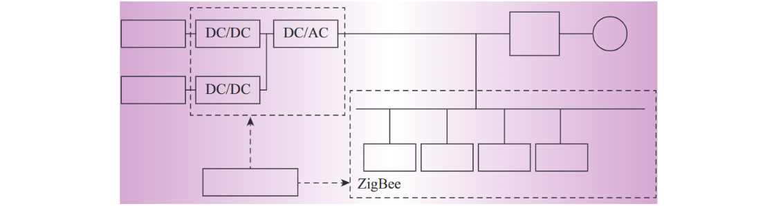
This paper designs a ZigBee - based smart home system, consisting of three components: home network, home server, and mobile terminal. The system is simple, efficient, and highly scalable, with its structure shown in Figure 1.

1 ZigBee - Based Smart Home Architecture
1.1 Home Network

As the core foundation, the home network connects controllable loads as nodes for internal data transmission and multi - energy management. Opting for wireless (ZigBee) over wired solutions boosts flexibility, reliability, and scalability.ZigBee, built on IEEE 802.15.4, offers low cost, power, and complexity with high security. Its affordable chips cut system hardware costs. The network includes:

Coordinator: Manages the ZigBee network (CC2530 - based, IAR - compiled), covering typical homes via direct - connected topology.
Terminal Nodes: Integrated with metering/relays (as smart sockets), collecting data and executing commands for “control + monitoring” closure.

1.2 Home Server

The server acts as the system’s “data - control core”, handling:

Data Hub: Exchanges info between ZigBee (via serial port) and mobile terminals (via Socket).
Operation Monitoring: Tracks load status, controls switches, and stores electricity data.
Energy Efficiency Brain: Analyzes load/photovoltaic data to optimize scheduling, closing the energy management loop.

1.3 Mobile Terminal

Android - based (Eclipse + Java), the terminal enables:

Status Visibility: Real - time display of server - pushed electricity info.
Remote Control: Sends commands to control loads indirectly.
Flexible Scheduling: Sets custom load timings (e.g., for time - of - use pricing).

2 Home Energy Efficiency Management Design
2.1 System Architecture & Logic

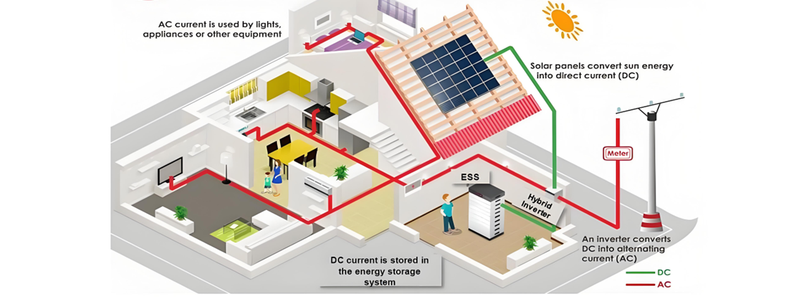
Integrating “smart home + PV + energy storage”, the system embeds efficiency strategies in the server, forming a “collect → model → optimize” loop:

Data Layer: Combines load and PV data.
Model Layer: Balances PV use, storage, and load via optimal schemes.
Control Layer: Coordinates PV/storage operations and load scheduling for “cost - efficiency” goals (structure in Figure 2).

2.2 Core Components & Collaboration

Key components (PV arrays, batteries, inverters, server, loads) work as:

PV Arrays: MPPT - enabled via inverters, transmitting real - time output to the server.
Energy Storage: Grid - connected, charging during PV surplus and discharging during shortages (metered for grid interaction).
Server: Links inverters/sockets, adjusting devices per efficiency rules to optimize energy flow.

2.3 Load Classification & Scheduling

Loads split into three types for time - of - use pricing - driven scheduling:

Critical Loads (e.g., lighting): Fixed - time, non - adjustable.
Adjustable Loads (e.g., AC): Variable - demand, power - tunable.
Shiftable Loads (e.g., washers): Time - flexible, core for efficiency.

The server controls shiftable loads via smart sockets, shaving peaks/ filling valleys to cut costs and stabilize the grid.

3 Mathematical Model and Control Strategy for Home Energy Efficiency Management
3.1 Mathematical Model for Home Energy Efficiency Management

To achieve precise home energy efficiency management, a mathematical model for total electricity cost must be established. This paper uses a “daily” control cycle, dividing 24 hours into

n

equal time intervals. By discretizing continuous problems (when

n

is sufficiently large, each interval approaches a “micro - element,” and variables can be assumed constant within the interval).In the

t

-th interval, based on the dynamic balance of “home load power, photovoltaic generation power, battery charging/discharging power, and grid interaction power,” the system power balance equation is derived as:

Within the

t

-th time interval, the power variables are defined as follows:

$P_{G t}$ : Grid interaction power (positive for power absorption, negative for power injection);
$P A t$ : Total household load power;
$P b t$ : Battery charging/discharging power (positive for discharge, negative for charging);
$P PV t$ : Photovoltaic (PV) output power (influenced by solar irradiance, temperature, humidity, etc., and predictable via PV power forecasting models).

The household PV system operates under the "self - consumption + surplus power grid - feeding" model, where surplus electricity generates grid - feeding revenue and PV generation qualifies for subsidies. Considering time - of - use (TOU) pricing (higher peak rates, lower off - peak rates), the total electricity cost is calculated as:Total Cost=Grid Purchase Cost−Grid - Feeding Revenue−PV Subsidies

For a daily cycle discretized into

n

intervals, the total cost model can be further decomposed into the summation of interval - specific costs, precisely adapting to dynamic pricing scenarios.

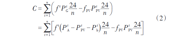
In the formula:

C

represents the total daily electricity cost of the household; f_PV is the unit price of the photovoltaic power generation subsidy;

24/n

is the duration of one time interval.
The expression for

f t

in Formula (2) is

In the formula:

f t

_Cis the electricity price for the user during the

t

-th time period, which is divided into peak - time electricity price and off - peak electricity price according to different time periods;

f R

is the electricity price for surplus electricity fed into the grid. The values of

f C t

f R

and

f PV

at any moment of the day are all known.The total power

P A t

of the household load is equal to the sum of the power of all shiftable loads and other loads during the

t

-th time period.

In the formula:

P L,i

is the operating power of the

i

-th shiftable load;

T L,i

is the start - up time of the

i

-th shiftable load; Δ

t i

is the operating duration of the

i

-th shiftable load;

[t i s, t i e]

is the range of the start - up time of the

i

-th shiftable load.

P L,i

, Δ

t i

t i s

and

t i e

are all definite values.

The electric power

P else,j t

of other loads is known, while the electric power of shiftable loads changes according to different start - up times, and

T L,i

is an undetermined value. When

T L,i

is different, the total power

P A t

of the household load changes accordingly, thus changing the total household electricity cost

C

3.2 Control Strategy

The core goal of home energy efficiency management is maximizing economic benefits, specifically translated into constructing an objective function for "minimizing the total household electricity cost

C

Based on the shiftable load model and combined with the time - of - use pricing mechanism, adjusting the start - up time

T_{\text{L},i}

of shiftable loads can dynamically optimize the total household load power curve, reducing the total cost from the perspective of electricity consumption timing.

Coordinated Control Logic for PV and Energy Storage

For photovoltaic (PV) power generation and energy storage batteries, control strategies are formulated for different time periods:

Peak Periods: Prioritize full consumption of PV power generation. If PV output > load power, surplus electricity is fed into the grid for revenue. If PV output < load power, the battery is prioritized for power supply (when the battery state of charge > minimum value). When the battery is depleted, the insufficient part is supplemented by the grid.
Off - Peak Periods: The battery is charged at the maximum charging power for energy storage. All load electricity is supplied by the grid, utilizing low - price off - peak electricity to "fill the valley" and store energy for peak periods.

Battery Constraints

It is necessary to simultaneously consider the charging/discharging power limits and capacity restrictions of the battery to constrain its charging and discharging behaviors (specific constraints need to be supplemented with formulas/models, not fully presented in the original text), ensuring equipment safety and system stability.

In Formula (6):

P b,max

is the maximum charging/discharging power of the battery; in Formula (7),

SOC t

is the state of charge (SOC) of the battery during the

t

-th time period;

SOC min

is the minimum value of the battery’s SOC;

SOC max

is the maximum value of the battery’s SOC.

According to the control strategy, optimize and control the charging/discharging power of the energy storage battery. During the peak period

t \in[t 1, t 2

, where

t 1

is the start time of the electricity peak period and

t 2

is the end time of the electricity peak period, the discharge power of the battery is set as

During the off - peak period

t \in [1, t 1]

, the discharge power of the storage battery is set as

It is necessary to calculate the state of charge (SOC) of the storage battery. The relationship between the state of charge during the charging and discharging process of the storage battery and the charging/discharging power is as follows:

Formula (10) describes the relationship between the storage battery’s SOC and charging power during charging (here

P b t ＜ 0

; Formula (11) describes that during discharging (here

P b t ＞ 0

SOC t + 1

is the SOC in the

t + 1

th period; σ (self - discharge rate, nearly 0% for small time intervals), η_ch (charging efficiency), η_$dis$ (discharging efficiency), and

E b,max

(max capacity) are battery parameters.In summary, home energy efficiency optimization aims to minimize total electricity cost by determining shiftable loads’ start times and energy storage charging/discharging power at each moment, stated as:

Objective function

Constraint conditions

4 Case Analysis

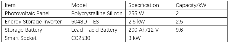
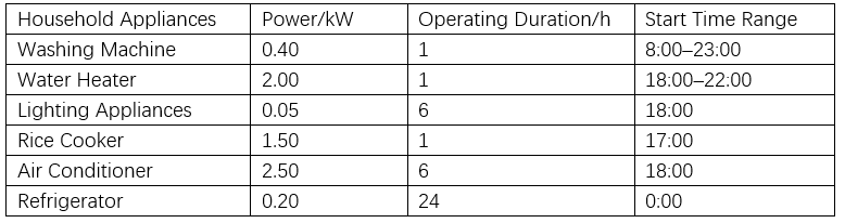
To verify the effectiveness of the proposed home energy efficiency management method, simulations and analyses are conducted using the household electrical equipment of a typical household in Shanghai. The home energy efficiency management system consists of photovoltaic panels, batteries, an inverter, a home server, and household loads. The system configuration parameters are shown in Table 1.

Shanghai implements time - of - use electricity pricing for residential living electricity, with peak hours from 6:00 to 22:00 at 0.617 CNY/kWh, and off - peak hours from 22:00 to 6:00 the next day at 0.307 CNY/kWh. The feed - in tariff for surplus PV electricity is 0.4048 CNY/kWh. Shanghai’s photovoltaic power generation subsidies include a national subsidy of 0.42 CNY/kWh and a local subsidy of 0.4 CNY/kWh, totaling 0.82 CNY/kWh.

Assume that the maximum charging - discharging power of the battery is 1.5 kW; the minimum state of charge (SOC) is set to 0.2, and the maximum is 0.9. The initial SOC

(SOC 1)

of the battery is set to 0.2; the charging - discharging efficiency of the battery is 0.9.

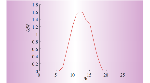
Set

n = 144

, dividing the 24 - hour day evenly into 144 time intervals, with each interval being 10 minutes. Figure 3 shows the power generation curve of the PV system on a certain day. The operation parameters of household loads are shown in Table 2, where the washing machine and water heater are shiftable loads.

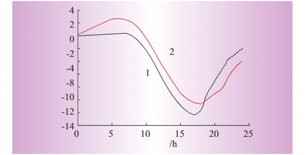
Based on the above data in Table 2, Matlab is used to conduct a simulation study on the optimal management of household loads. According to the home energy efficiency management algorithm, the optimal household electricity usage scheme is determined to minimize the total daily electricity cost. The simulation results are shown in Figure 4.

After simulations, the minimum total household electricity cost occurs when

T Li1 = 133

and

T Li2 = 132

(washing machine starts at 22:00, water heater at 21:50).

Figure 4 shows the daily cost curve. Curve 1 (no energy management) and Curve 2 (with load shifting and storage control) reveal: Negative costs mean grid - feed revenue + PV subsidies > grid costs. Post - 6:00, PV growth cuts costs until 17:00 (PV drops to 0, grid supply raises costs), ending at

C = -2.02

CNY at 24:00.

With energy management, Curve 2 shows: Post - 0:00, battery charging (from grid) boosts costs fast. Post - 17:00, battery supply slows cost growth vs Curve 1. Load shifting further reduces costs, ending at

C = -4.10

CNY (a 2.08 CNY decrease).Simulations confirm the algorithm works—cutting costs, improving economy, and achieving peak - shaving.

5. Conclusions

A ZigBee - based smart home system integrating PV, storage, and energy management is designed. A mathematical model and time - of - use pricing - based algorithm are built. Simulations show it optimizes storage charging/discharging and load timing, slashing costs, boosting benefits, and proving feasibility.